Length and Area Estimation in Images

More and more of our daily activities are becoming automated and digitized. Current technology relies a lot on computer data and its processing to make efficient decisions and solutions. Few of such technologies involve optical sensing devices and smart camera systems. These technologies revolutionized the way we look at things from the very small to those that exceed our human proportions by orders of magnitude.

In the field of medical technology, image processing is a milestone for capturing live and real time images of minute cells. In space exploration, we have estimated the areas of the craters of the moon, approximated the heat of the sun, and even counted the very stars that made our heavens.

This \(blog post\) is a taste of those applications in a VERY simplified manner. Same concepts, same math, minus the proportions.

There are a lot ways in which an area can be estimated given an image. The most basic and most rigorous approach would be directly counting the pixels that lie within a boundary and by sorting out the pixels by the magnitude of its intensity. But that’s only one way of doing it. A more ‘mathematical’ and ‘elegant’ approach is by using Green’s Theorem (recall basic Calculus). This theorem basically relates a double integral to a line integral [1]. #test

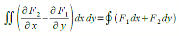
For some continuous function \(F_{1}\) and \(F_{2}\) (with continuous partial derivatives) that contains a region \(R\), Green’s Theorem relates that:

Suppose that \(F1=0\), \(F2=x\) and \(F1=−y\), \(F2=0\), then at the region \(R\) and at the contour boundary \(C\), the equation above becomes,

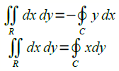
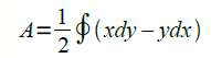
These double integrals give us the area of the region \(R\) to the right and to the left, respectively. Adding the two,

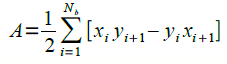
In discrete form,

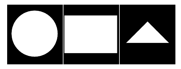
For the first part, I used Green’s Theorem to find the area of regular shapes. Using Scilab, I generated a circle with radius of \(0.7 units\), a rectangle with length \(1.4 units\) and width \(1 unit\), a triangle with height \(0.5 unit\) of and base of \(1 unit\). Shown below are the synthetic images.

Before we can apply Green’s Theorem, the edge of the shapes should be determined first. In Scilab, the module SIVP (Scilab Image and Video Processing toolbox) has five readily available edge detection algorithms [2]:

sobel

Detects edges, using the sobel gradient estimator. It isbased on convolving the image with a small, separable, and integer-valued filter in the horizontal and vertical directions [3].

prewitt

Detects edges, using the prewitt gradient estimator. Technically, it is a discrete differentiation operator, computing an approximation of the gradient of the image intensity function [4].

log

Detects edges, using the the Laplacian of Gaussian method. sigma (default: 2) is the standard deviation of the Log filter and the size of the Log filter is nxn, where $$n = ceil(\sigma*3)*2+1$$

fftderiv

Detects edges, using the FFT gradient method, (default: sigma = 1)

canny

Detects edges in *im*, using Canny method. *thresh* is a two-element vector, in which the fist element is the low threshold and the second one is the high threshold. If *thresh* is a scalar, the low threshold is $$0.4*thresh$$ and the high one is *thresh*. Besides, *thresh* can not be negative scalar. sigma is the Aperture parameter for Sobel operator, which must be 1, 3, 5 or 7; (default: thresh = 0.2; sigma = 3).

Green theorem is then applied to the edges of the shapes with the following code:

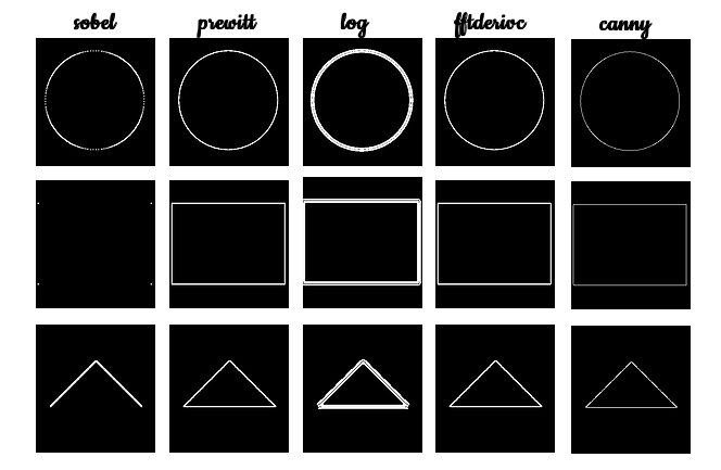
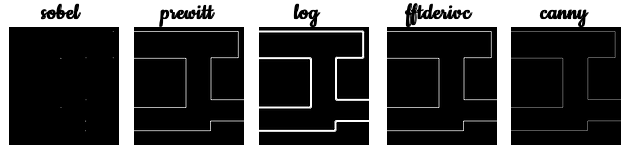
The comparison of how the five edge detection algorithms performed is shown,

Below is a table showing the summary of the results of the calculated area of the shapes using Green’s theorem with different edge detection algorithms.

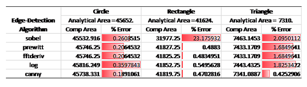
From visual inspection of the images, the prewitt, fftderiv and canny produced the thinner and more accurate edge detection compared to the others. These visual comparisons are backed up by the low percent error of the computed area to the analytical area of the shapes as can be inferred from the Table. Overall, the canny algorithm seems to outperform all the other given that it produced the least error value.

To test this, I went to Google Earth (left) and Google Maps (right) and searched my beloved dormitory in UP (Yakal Residence Hall). The images below show the satellite view of the dormitory.

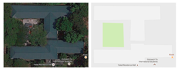
I uploaded the Google Maps image to Paint (Microsoft), whiten the area of the building and blacken everything else as shown:

Applying Green’s Theorem to find the area and comparing the five edge detection algorithms, the results are as follow:

The table below shows the summary of the results of the calculated area of the shapes using Green’s Theorem with the five different edge detection algorithms.

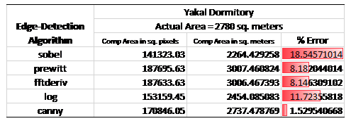
I found the actual area of the dormitory by getting the convex hull of the building in Google Maps. This is done by getting the smallest number of points to enclose the area. Google automatically calculated the area for me, so no sweat. The table above is fairly consistent from the results of the regular shapes. Indeed the canny algorithm bested the other four. The offset of the canny method to the actual area is about \(43 m^2\) which is roughly about four standard rooms. Not bad for my purpose of approximating areas with Green’s theorem. Most errors would come from me being a human huhu i.e. misaligning in covering area in Google Maps.

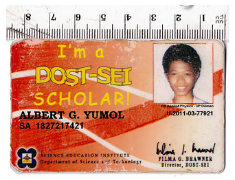
For those people who want to skip rigorous math and don’t have much time, an alternative method is by using ImageJ and a straight edge. I scanned my decade old DOST ATM card together with a reference ruler (for scaling and direct measurement). I definitely look older 10 years ago.

I uploaded this image to ImageJ, a free open source software for measuring microscopic images. I drew a straight line across the horizontal and set the scales as shown:

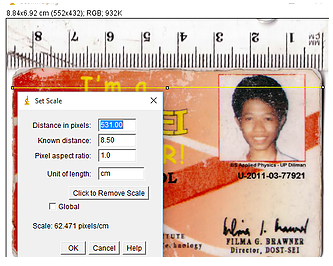
After setting the scales, I know that the area of my card is \(45.9 cm^2\) by physical measurements. I then used the free hand selection tool to draw a polygon that fits around the sides of my card. I clicked the measurements and it gave an area of \(45.842 cm^2\) which is \(0.12%\) away from the actual value. It was accurate enough even though I was not even making tremendous effort on making the shape really fit the sides line to line. ​ Want to collaborate? Message me in LinkedIn.

References:

[1] M. Soriano, “Length and Area estimation in images,” Applied Physics 186 Activity Hand-outs, 2014.

[2] Scilab Image Processing. Retrieved from: http://siptoolbox.sourceforge.net/doc/sip-0.7.0-reference/edge.html

[3] Wikipedia. Sobel Operator. Retrieved from: http://siptoolbox.sourceforge.net/doc/sip-0.7.0-reference/edge.html

[4] Wikipedia. Prewitt Operator. Retrieved from: http://siptoolbox.sourceforge.net/doc/sip-0.7.0-reference/edge.html

[5] Barteezy’s Applied Physics Experience. Retrived from: http://siptoolbox.sourceforge.net/doc/sip-0.7.0-reference/edge.html