Properties and Applications of the 2D Fourier Transform

It has been demonstrated in the previous activity, the definition and basic applications of the Fourier Transform (FT). Different apertures (or FT operations) based from the corresponding image were produced and compared. Convolution and correlation was successfully utilized and performed for 2D signals and lastly, an edge-detection technique was implemented using the FT.

This next activity is all about the properties and applications of the 2D Fourier Transform.

Anamorphic Property of FT of Different 2D Patterns

In the FT process, a signal of X dimension transforms to a 1/X dimension. This means that if a signal appears wide on an axis, it will appear narrow in the spatial frequency axis. This property is called anamorphism.

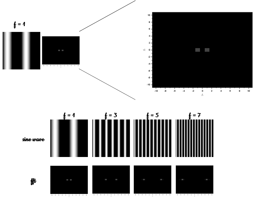
The first part of the activity is demonstrating the anamorphic property of FT for different 2D patterns; (a) tall rectangular aperture, (b) wide rectangular aperture, (c) two dots along the x-axis symmetric about the center, and (d) same as (c) but with different spacing of the dots. The results are shown below:

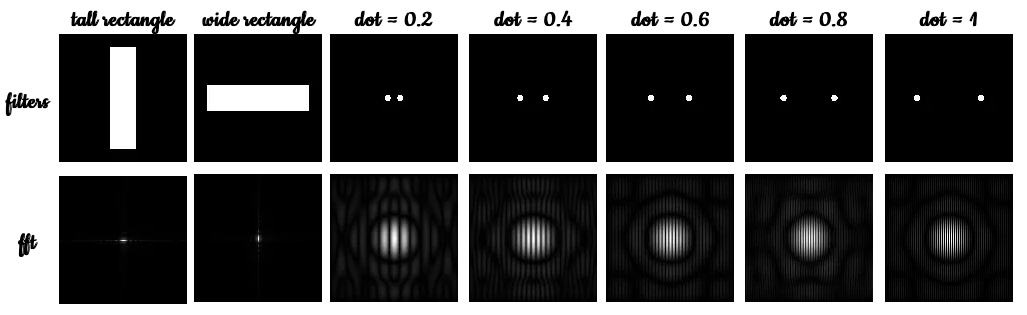
For both the rectangle filters, we see that in frequency space, small dimension will be mapped as large dimensions. The tall rectangle will have dominant intensities along the horizontal axis while the wide rectangle will have dominant intensities along the vertical axis. The dots on the otherhand, approximate two direc deltas. The FFT of two points is a sine wave while the FFT of a small circle is an Airy pattern. Thus, the FFT of two points separated by a distance exhibits both the Airy pattern and a sine wave.

As the distance of the dots are increased, the frequency of the sine wave in Fourier space also increases (or decreasing width of the bands) which we have already established as anamorphism. The operation that governs this transformation is simply the convolution process that was discused in Activity 5 and will be elaborated later.

Rotation property of the Fourier Transform

Recall from Activity 3 how we generated the corrugated roof or a sinusoid along the x-axis. Below are images of the corrugated roof with varying frequency together with their FFTs, recall Activity 5 on how we get the FFT of the corrugated roof.

The images above tells us that as the frequency of the generated sinusoid is increased, the distance of the corresponding dirac deltas in the frequency space also increases.

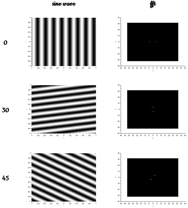
The next part is rotating the sinusoid z below by introducing an angle, z is given by:

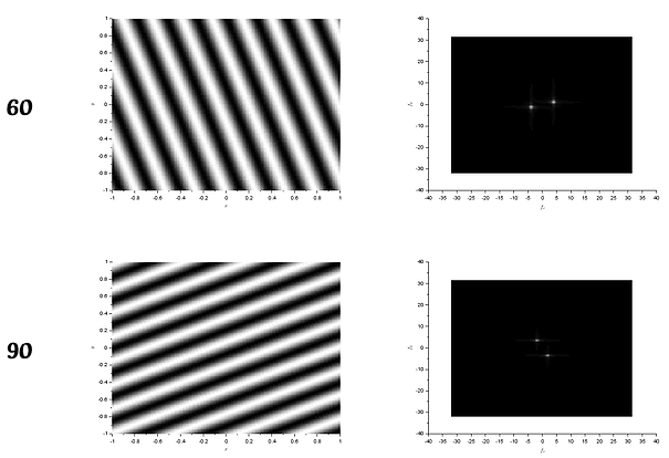
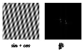
The results of the rotation of the sinusoids tells us that the acquired FT is also rotated with the corresponding angle. The frequency, or the separation distance of the dots were still the same no matter what rotation. One can also play with the combinations of sinusoids. For example, adding a sine and cosine with different frequencies (4 and 6) and angle of rotation (30 and 45),

These combinations are governed by trigonometric relations and thus one can predict the location of the FFT dots by just looking the at frequency and and angle of rotation of the waves.

Convolution Theorem Redux

Practical application of FT is on masking techniques. Noise (unwanted) or repetitive patterns in an image can be removed by filtering these frequencies in Fourier space. This masking can be accomplished by using a filter which is simply a convolution operation. Recall from Activity 5 that the FT of a convolution of two function f and g is just the product of the two functions FT.

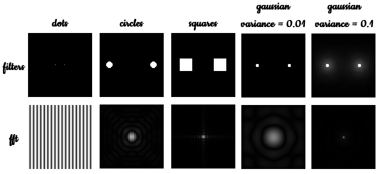
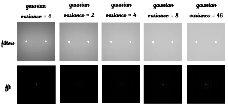
In this next activity, we first demonstrate the FT properties of different filters; two dots, two circles, two squares and two gaussian dots with different variance. Shown below are the filters together with their FFTs:

For the two dots, we still observe that its FT is still a siunsoid along x. When replaced by two circles, we observe an Airy patterns with a corrugated roof inside it. In essence, the resulting image is just the multiplication of the FT of two dots and the FT of a circle. This observation holds for all filters as in a square and a gaussian.

For the gaussian profile, as the variance is increased, the Airy pattern becomes less and less apparent and finer. All thanks to anamorphism and convolution. It is also demonstrated that indeed the FT of a gaussian is still a gaussian.

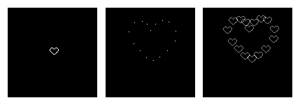
As an application of this observations, I generated a 200x200 image with 16 dots arranged to form a heart shape. Next, I created a heart pattern and convolved the two images. The results are shown below. Indeed the convolution is just the product of their FT’s such as in the correlation exercise in Activity 5.

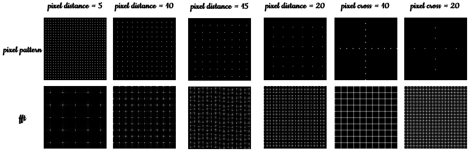
Moving on to the next part, we observe the FT of repeated patterns. In Scilab, I generated pixel patterns with different spacing. I obtained their FTs and the resulting images are as follows:

To interpret the results, we can treat a square grid as symmetric dots in x and y axis. The FT of these dots are sinusoids summed together as seen in the FTs of the pixels above.

Because of anamorphism, as the pixel distance is increased, less dots will form on the grid and thus will form more points in the Fourier space.

Fingerprints : Ridge Enhancement

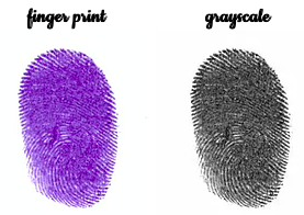
The next demonstrations are on the practical applications of FT filtering. I prepared my own finger print and converted it to grayscale using Scilab:

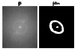
I then obtain the FFT of the grayscale image and made a filter that is the same size as the original image. The FT and the filter are as follows:

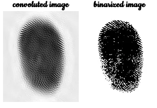
The high intensity lines of the FFT of the fingerprint represents the ridges. By multiplying the images above to acquire the convoluted images as shown below:

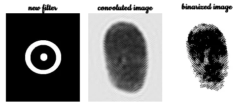
The ridges became more apparent but their are still blotches. I tried another filter and repeated the whole process:

There is an improvement in the visibility of the ridges. But the blotches are still apparent. NOT UNTIL NOW HAVE I REALIZED MY MISTAKE. I have made a very large filter at the center. For the mean time, the very least I have demonstrated ridge enhancement of the sides of my finger print. I will definitely update this very soon.

Lunar Landing Scanned Pictures : Line Removal

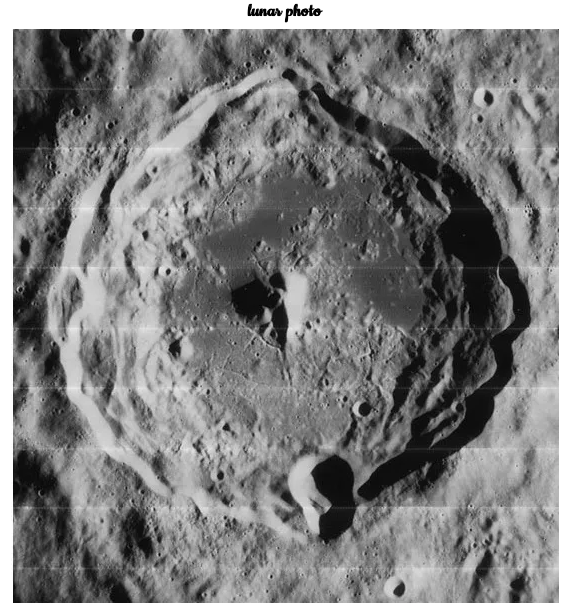
The next application of noise reduction using FFT is filtering unwanted patterns in frequency space. The image chosen was a lunar surface photo presumably from NASA given below.

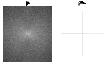
Same as what I did for the finger print data, I obtained the FFT of the image and made a corresponding filter as shown below:

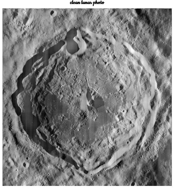
Multiplying the two images to obtain the convoluted image, I get the result:

Indeed, FT filtering is effective in cleaning images with line patterns due to image stitching.

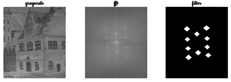
Canvas Weave Modeling and Removal

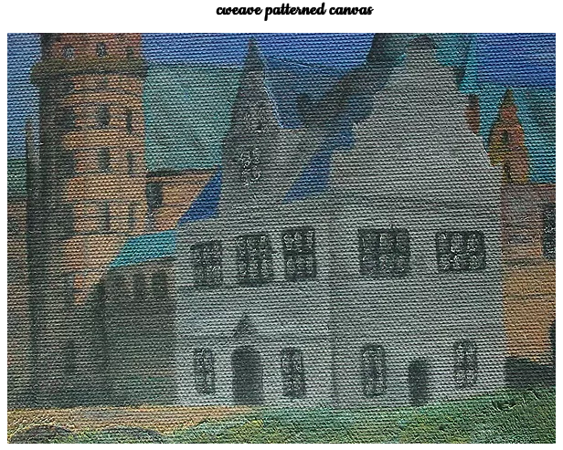
This last application of FT removal is a little bit tricky. The image is an art canvas with weave patterns. The challenge is to remove the weave patterns. This is easy because it requires exactly the same process as was done in the finger print and lunar photo. The challenge is how to render the image in full color. The image is shown below:

I first separated the image in grayscale and the corresponding color channels: red, blue and green. I obtained the FFTs of the different channels, convolved it to the filter.

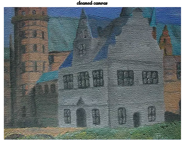
Using the flipdim() function in Scilab, I was able to render and combine the color channels to one image. The resulting image is shown below.

In summary, I have explored the properties and applications of the 2D Fourier Transform. Content-wise this activity proved to be the longest and tiring so far. But all the effort was worth it. Image processing indeed is an intricate subject. You get to learn a lot things by doing, making mistakes, and learning from those mistakes. I spent almost three weeks to finish the activity trying to learn the processes and debugging the code. I hope that I may be able to build upon my basic knowledge of FT filtering for my future scientific endeavor.

Want to collaborate? Message me in LinkedIn.

Reference:

[1] M. Soriano, “Properties and Applications of the 2D Fourier Transform,” Applied Physics 186 Activity Hand-outs, 2014.