Fourier Transform Model of Image Formation

Throughout my physics ‘career’, there is one mathematical ‘trick’ that always haunts me. Be it signal analysis, optical systems, acoustics and of course image processing, this ‘trick’ is omnipresent. You probably know what I mean more or less if you have encountered these topics and have taken some applied mathematics courses before. I am talking about the all famous and magnanimous Fourier Transform (FT).

My ears still ring of the monotonous tone of my signal processing professor saying that “everything is just a signal that can be described as a series of sines and cosines”. Every scientist and engineer, before they get their degrees will have to master FT one way or another.

The Fourier Transform (FT) was formulated by Joseph Fourier in 1822 [1]. He showed that a lot of mathematical functions could be represented as a sum of sines and cosines. Physically, FT converts a signal in \(X\) dimension to a signal in \(1/X\) dimension. Given an image \(f(x,y)\), the FT is defined as:

where \(f_x\) and \(f_y\) are spatial frequencies along \(x\) and \(y\) respectively [2]. We can treat the FT process as analogous to a simple lens system. As light from an object passes through an aperture, an inverted image of the that object is formed in the image plane. The FT operation can be treated as the aperture of the lens system.

In numerical calculations and simulations, the easiest way (from my experience that is) of implementing FT is the Fast Fourier Transform (FFT) developed by Cooley and Tukey. Almost all high level programming languages have modules for implementing the mighty FFT.

Familiarization with discrete FFT

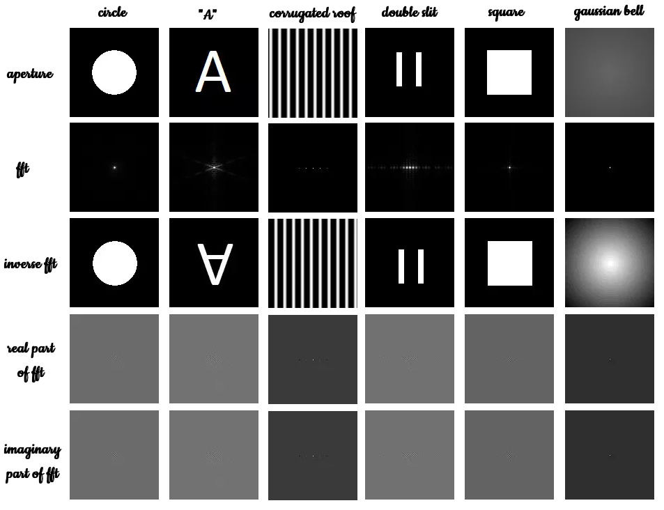
In this post, we will compare different apertures (or FT operations) and explore on two FFT operations, namely convolution and correlation for 2D signals. At the end, we will apply these methods to an edge-detection algorithm. The image Shown below is the summary of the results for different apertures.

The goal is to find the fat of a circle, the letter A, sinusoid along the x-axis (corrugated roof), a double slit, a square and a gaussian bell curve. The circle, the corrugated roof, the square, and the gaussian bell curve were generated with scilab while the letter A and the double slit was manually drawn in paint. All of the synthetic images are all 128x128. If you are interested on how to generate some of these synthetic images in scilab, click here for Activity 3: Scilab Basics.

We start first with the basic circular aperture. After importing the image, it was converted to grayscale so that we can discretize the image intensity values from 0 to 255. FFT is then is performed to the image using fft2() for two dimensional fft.

The FFT operation outputs complex numbers so the abs() function is used to get the magnitude. Remember as well that in FFT, the diagonal quadrants of the image are interchanged. To correct this, the fftshift() is used.

To check if correct transformation was successful, the inverse FFT of the acquired image is obtained. Theoretically, the output from this operation should be the same values as the input image only inverted. Real and imaginary values of the images are also shown below.

From the FFT of the circle we see that it is composed of concentric circles with densities higher at the centre. This pretty pattern is often termed as the Airy Pattern. In this case, image inversion cannot be discerned since the a circle is both symmetric in the x and y axis.

Zooming in to this image we clearly see alternating dark and bright bands that we call fringes. This pattern can be explained by the action of constructive and destructive interference as in optical imaging systems. Since “light” converges at the focal point (centre of the aperture), the most intense or the whitest part should be seen at the centre.

Generally we see the same features for the other apertures. For the letter A, its FFT were translated horizontally. This is because in FFT operation we observe the image in the spatial frequency domain or 1/X dimension. The letter A is chosen to easily discern the image inversion and and the transformation from X domain to 1/X domain.

The next aperture is the corrugated roof pattern (sinusoid along x). Again, an airy pattern is observed. In the FFT of the image, the intensity is highest at the centre since the parallel rays converge to the focus. This patterns can be interpreted physically as the location of the spatial frequency of the signal since the aperture is a sinusoid.

The next aperture is the famous double slit pattern. This is so cool. We have just confirmed Young’s experiment using Scilab! Obviously we would observe an interference pattern from the FFT of the double slit. From the results, we see that the interference patterns occurs both at the horizontal and vertical axis.

Almost similar results were obtained for the square aperture as compared to that of the circle with exception of the shape of the acquired image.

The last aperture is the gaussian bell curve with sigma = 0.9. Theoretically, the FFT of a gaussian is still a gaussian. Indeed, we see that the FFT of the gaussian is a seemingly small that when zoomed resembles a gaussian. The smaller size of the image can be attributed to the decreasing intensity of the gaussian aperture.

Convolution

The next part of the activity is using FFT in the convolution process. Basically convolution is just multiplication in frequency space. The convolution between 2D functions f and g is given by,

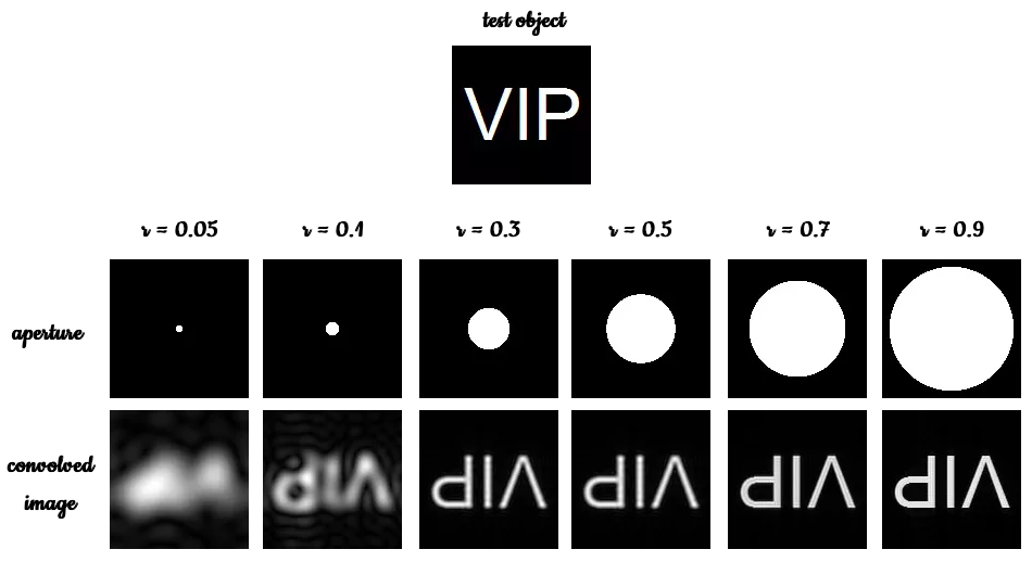
But for what purpose does the FFT serve convolution? Apparently, it was found out that the convolution of two signals is just the inverse FT of the product of these two signals’ FT. To demonstrate this relation, we consider two images; a circular aperture and the word “VIP” (shorthand for Video Image Processing). The two images serves as the two functions to be convolved. Shown below is the summary of the results with varying radius or aperture sizes,

As we can infer from the images above, the is a direct effect to the output image when the aperture size is varied. As the aperture size is increased the output image becomes more crisp meaning that the edges are more apparent. This is because the FT of smaller circular aperture produces more Airy pattern causing a blurry output when used in convolution. For a larger aperture, the FFT converges into a spot, making the output image crisp and clear.

Correlation

The next part of the Activity is on signal correlation. Correlation is an operation that determines the degree of similarity between two signals. For 2D functions, the correlation is given by,​

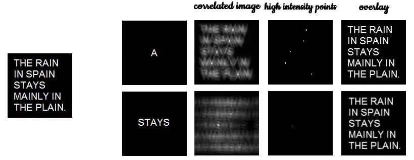
where p is the correlation of signals f and g. The value of p is close to 1 at a particular location if the two signals f and g are similar at that location. Apparently, it was found out that the correlation of two signals is just the inverse FT of the product of the FT of G and the conjugate of the FT of f. To illustrate this, the image “THE RAIN IN SPAIN STAYS MAINLY IN THE PLAIN” is correlated with the letter A.

In the third column of images above, we see the correlation of the two images. The high intensity dots represents region of high correlation, meaning the letter A can be found at those particular locations. Figure b is the mapping of those high intensity points. Overlaying the original image and the mapped points,we see that indeed, successful correlation of the two images. To demonstrate it further, the word “stays” was used and correlated to the original image. We see that the again the high intensity spot correspond to the location where the word “stays” can be found.

Detection

The last part of the Activity is edge detection techniques using the Fourier Transform. In edge-detection, a template pattern is usually used and matched with an image. This template is generally a 3x3 matrix with an element sum of zero. The “VIP” image is used and convolved to the 3x3 matrix with different combinations. Before convolving the two, the 3x3 matrix was first converted to the same size as the “VIP” image which is 128x128. This was done by surrounding the 3x3 matrix with zeros. The results are as follows,

As we can see from the results, the horizontal edges was detected by the horizontal matrix. This is true to all types of matrix combinations. By inspection, the best edge detection matrix would be the center or the cross. It is also good to note that the edge-detection technique used in SIVP like sobel, prewitt, log, fftderiv and canny employs the same type of matrices but of different element distributions.

Another interesting insight is that the sign is a very important factor in the distribution of the elements. All my code can be found here.

In summary, we have compared different apertures (or FT operations) based from the corresponding image produced. Convolution and correlation was also successfully for 2D signals and lastly, an edge-detection technique was implemented using the FT.

I have gained a lot more insights on how useful FFT really is. I am looking forward to more applications of FFT to my research on signal analysis and processing.

Want to collaborate? Message me in LinkedIn.

References:

[1] Wikipedia. Fourier Transform. Retrieved from: https://en.wikipedia.org/wiki/Fourier_transform

[2] M. Soriano, “Fourier Transform Model of Image Formation,” Applied Physics 186 Activity Hand-outs, 2016.

[3] Barteezy’s Applied Physics Experience. Retrived from: https://barteezy.wordpress.com/2015/09/19/activity-5-fourier-transform-model-of-image-formati/