![[Developing] Basic Statistics Review for Data Science](/images/stat/normal.png)

[Developing] Basic Statistics Review for Data Science
This is a draft for basic statistics module for data scientists developed for Eskwelabs. The module assumes that the reader knows some basic Pythons and survival algebra.
Outline
- Measures of Central Tendencies
- Measures of Dispersion
- Covariance, Correlation, and Causation
- Probability
- Dependence, Independence, and Conditional Probability
- Bayes’ Theorem
- Random Variables
- Continuous distributions
- Normal distribution
- Central Limit Theorem
- Hypothesis and interference
- Confidence interval
- Bayesian inference
In the recent decade, we have produced majority of our data due to the increase in computing powers of our machines, increase in volume of our storage systems and the decrease in the production cost of technology. These led to the accessibility of technology to a lot more people.
But data is just that - data. It doesn’t really tell us much. To get insights from it, we need to process it.
Take as an example the qualifying entrance exam for Eskwelabs. Assume that there are 50 items for the exam with 100 examinees. You have already learned by now how to generate synthetic data in Python. Now we generate the scores randomly and visualize using a bar plot hoping that no one scores below 50.
Here is how you do it in Python:
And here is the resulting distribution:
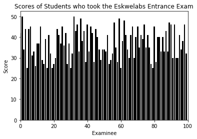
Visualizing can give us a feel of what the data looks like. We can see that one student actually perfected the exam (maximum) and the lowest score is around 25 (minimum). From these we can tell that the scores ranges from 25-50.
Most of the time, visualizing data is not enough to get insights. That is where statistics comes in.
[Statistics][1] refers to the mathematical methods and techniques to gain insights from data. I know you already did some statistics before. So this should be easy breezy.
The three most common tool used in data description is what we call the measures of central tendency.
Measures of Central Tendencies
In exploring our data sets, we want to check the average or central values of our data. Centrality can be measured by these 3 values: mean, median, and mode.
Mean
The mean gives you an initial summary of your data set. It is obtained by getting the sum of the individual data points \(x_{i}\) and divide this sum by the total number of data points \(N\).
Mathematically:
\[\begin{equation} \overline x = \sum_{i}^{N} \frac {x_i}{N} \end{equation}\]Programmatically in Python:
Calculation the mean exam scores of Eskwelabs applicants, we find that the average score is \(36.9\) which is \(73.8%\). Not bad if the exam is difficult. This value somewhat gives us an idea of how the examinees performed overall in the exam.
Another measure of central tendency is the median.
Median
The median is the middle value of the data set when you sort out every single points from lowest to highest. The most common approach in obtaining the median value is by considering two cases: when the length of data set \(N\) is odd or even.
When \(N\) is odd, it is not divisible by two thus we obtain a unique middle value.
Mathematically:
\[\begin{equation} M_{odd} = \left( \frac {N+1}{N} \right) ^{th} term \end{equation}\]The other case is when \(N\) is even which implies that there are two candidate values for the median. What you do is get the average of these two points.
Mathematically:
\[\begin{equation} M_{even} = \frac {\left( \frac {N}{2} \right) ^{th} term + \left( \frac {N}{2} + 1 \right) ^{th} term}{2} \end{equation}\]Implementing both these equations in Python:
If you are keen enough to notice, in our mathematical equation for the even case we add 1 to the middle value but when we implemented in code we change it by subtracting one. This is because in Python, we start counting from 0 so we need to account for this translation.
The median score for the Eskwelabs exam data set is 37 which is not far from the mean. As we have observed, the median is a bit more complex to calculate because you need to sort first and find the middle value. There are other approaches for median calculation without the tedious sorting. See this link for exploration: Sorting Less Median Calculation.
Although the mean is easier and faster to calculate, it is very sensitive to outliers unlike the median. So if your analysis requires less sensitivity to noise, median is the better descriptor.
As a side note, the median is a special type of measurement called quantiles. These refers to the partitioning of the data set in equal proportions. The median is actually a second order quantile because it divides the data set into two. Here is the general code to calculate the quantile based on order (or number of partitions):
The last measure of central tendency is the mode.
Mode
The mode is a measure of frequency. It gives you the most frequent value in your data set. You can use this to check the balance of your data set if it is biased for particular values. It can have more than one value if there is a tie for the maximum number of counts. The mode requires no formula since it is just the most frequent data point. One cool approximation for the mode by Professor Karl Pearson is given by the empirical formula:
\[Mode = 3(Median) - 2(Mean)\]For the Eskwelabs exam problem, the mode is:
Measures of Dispersion
Dispersion is the measure of the spread. It tells you the difference in values across all data points. A small dispersion value indicates the data points are near each other while a large dispersion means data points are far apart.
Basic dispersion measures include the range, variance, standard deviation, and interquartile range.
The range is self explanatory. It provides you the upper and lower bound of your data set. Mathematically:
\[Range = x_{max} - x_{min}\]In Python,
The problem with the range is that it is only describing the end points of the data set. It doesn’t provides us insights on the whole data set between in. To address this, we consider the next metric called variance.
Variance measure how far the data points are spread from the mean. Mathematically:
\[\sigma ^{2} = \sum \frac {x_i - \overline x}{N}\]where \(x_i\) is a single data point, \(\overline x\) is the mean, and \(N\) the total number of data points.
To do it in Python,
The variance will help us determine the size of the data spread but the problem is the units. The units for the measures of central tendencies and range are all the same but variance is in squared units. It will make more sense if we get the square root variance (same unit with the other measures) and we call it the standard deviation given by
\[\sigma = \sqrt {\sigma ^{2}} = \sqrt {\sum \frac {x_i - \overline x}{N}}\]In Python,
The standard deviation measures the absolute variability of the dispersion with respect to the mean. However, like the range it is also very susceptible to outliers. Depending on applications, a better metric would be the interquartile range. This can be calculated from the difference of \(75^{th}\) and \(25^{th}\) percentile value. In python,
Covariance, Correlation, and Causation
Statistics has also some philosophical roots. We often hear the phrase, ‘correlation is not causation’. Use correlation with a grain of salt. You may be mislead by simplified assumptions and confounding variables.
For example, if there exists a strong correlation between variables x and y, we conclude:
- x causes y
- y causes x
- both causes each other
- neither causes each other
Recall that the variance is a measure of how a single variable deviates from the mean, a covariance measures the variation of two variables with respect to each other and their means. Mathematically:
\[\sigma_{xy} = \frac {1}{N} \sum_{i} (x_i - \overline x)(y_i - \overline y)\]In Python,
The multiplication factor from the equation above is a dot product of two variables. A significantly positive covariance indicates that x is large when y is large and vice versa. A significantly negative covariance indicates that x is large when y is small and vice versa. A zero covariance indicates that there is no relation between the two variables.
We are now faced with the problem of interpreting the variance. Typically it is difficult to set how big a number is to be significant relative to other values. Another problem is the units, in this example x-units-y-units-per-unit-time. That is why we transform the covariance by normalizing it with the standard deviations of both variables \(x\) and \(y\). We call this transformed metric the correlation \(\rho_{xy}\) mathematically as:
\[\rho_{xy} = \frac {\sigma_{xy}}{\sigma_{x} \sigma_{y}}\]In Python,
This value is unitless (since we normalized) and ranges from [-1, 1]. We interpret values as:
-
1 : perfect correlation
-
0 : no correlation
-
-1 : perfect anti-correlation
Exercises:
(1) Generate two random samples: x ~ N(1.78,0.1) and y ~ N(1.66,0.1).
(2) Compute \(\overline x\), \(\sigma_{x}\), \(\sigma_{y}\), \(\sigma_{xy}\), \(\rho_{xy}\) from scratch (without using any module e.g. numpy, statsmodels). Compare the results with the ones from the numpy library and state your observations.
For further reading:
Python related:
Statistics Books and references:
Probability
Probably one of the hardest concept to grasp in statistics is probabilities. As humans we feel discomfort when confronted with uncertainty.
But for this brief tutorial we will not be dealing with the philosophical interpretation of probability. Those topics are more suitable for sober drink with geek friends.
Think of probability as our way of quantifying chance or uncertainty. It answers ‘What are the odds that an event \((E)\) will occur given all possible outcomes?’. We denote this statement as the probibility of E occurring: \(P(E)\).
Probability is one of the pillar concepts in Data Science. This is me implicitly telling you (or obliging you) to seriously appreciate this as we will use it to build models, train models, evaluate models, and a whole lot more.
Dependence, Independence and Conditional Probability
Consider two events \(A\) and \(B\). When knowing whether \(A\) happens gives us no information if \(B\) happens, we say that \(A\) and \(B\) are independent.
Mathematically,
\[P(A,B) = P(A)P(B)\]On the contrary, if knowing event \(A\) adds information if \(B\) occurs, we say that \(A\) and \(B\) are dependent.
Mathematically,
\[P(A | B) = \frac {P(A,B)}{P(B)}\]This is the definition of the conditional probability. We read this equation as the probability of the event \(B\) will occur given the knowledge that event \(A\) has already occurred. Or simply: probability of \(B\) given \(A\).
The conditional probability equation is the generalization of independent and dependent cases. This means that you can apply the equation to both cases.
Take note for this equation that it is only valid when \(P(A) > 0\) (because maths don’t permit division by 0).
The most common example to demonstrate this is the boy-girl problem. Consider a family with two children whose gender (birth) is unknown, the probabilities are as follows:
- no girl: \(\frac {1}{4}\)
- 1 girl, 1 boy: \(\frac {1}{2}\)
- 2 girls: \(\frac {1}{4}\)
Note that the sum of the probabilities of all events should be 1.
We assume that the siblings are not twins and the likelihood of a child being a girl and a boy is equal. We also assume that the gender of the second child is independent from the gender of the first child.
Consider two problems:
Problem 1: Find the probability of both children being girls (\(\alpha\)) given that the older child is a girl (\(\beta\)).
Problem 2: Find the probability of both children being girls (\(\alpha\)) given that at least one children is a girl (\(\gamma\)).
We start with all the possible outcomes:
- BB
- BG
- GB
- GG
To approach Problem 1, recall the conditional probability:
\[P(\alpha | \beta) = \frac {P(\alpha,\beta)}{P(\beta)}\]For this case \(P(\alpha,\beta)\) is just \(P(\alpha)\). Thus,
\[P(\alpha | \beta) = \frac {P(\alpha)}{P(\beta)} = \frac {\frac {1}{4}} {\frac {1}{2}} = \frac {1}{2}\]For Problem 2, \(P(\alpha,\gamma)\) is also \(P(\alpha)\). Thus
\[P(\alpha | \gamma) = \frac {P(\alpha)}{P(\gamma)} = \frac {\frac {1}{4}} {\frac {3}{4}} = \frac {1}{3}\]To do this numerically in Python, we can generate one million such families and confirm the probabilities.
The result are as follows:
- Problem 1: 0.4992346188401824 ~ \(\frac {1}{2}\)
- Problem 2: 0.3331819838973103 ~ \(\frac {1}{3}\)
Bayes's Theorem
Recall that conditional probability tells as that event \(\alpha\) occurs given \(\beta\). But what if we want to know the occurrence of \(\beta\) given only the probability \(\alpha\) given \(\beta\).
Let’s do some mathematical derivations :)
Conditional probability states that:
\[P(\alpha | \beta) = \frac {P(\alpha,\beta)}{P(\beta)}\]getting the inverse:
\[P(\beta | \alpha) = \frac {P(\beta,\alpha)}{P(\alpha)}\]we get,
\[P(\beta,\alpha) = P(\beta | \alpha)P(\alpha)\]using commutative property:
\[P(\alpha | \beta) = \frac {P(\beta,\alpha)P{(\alpha)}}{P(\beta)}\]Next we split \(P(\beta)\) as:
\[P(\beta) = P(\beta, \alpha) + P(\beta, \alpha ^{\dagger})\]The \(\dagger\) indicates ‘not occurring’.
Substituting the variables and applying the conditional probability equation we get:
\[P(\alpha | \beta) = \frac {P(\beta | \alpha)P(\alpha)}{P(\beta | \alpha)P(\alpha) + P(\beta | \alpha ^{\dagger})P(\alpha ^{\dagger})}\]Famous example:
The medical doctor vs. The Data Scientist
Imagine a scenario of true positive test in a data set. Suppose that 1 every \(10,000\) people have a disease. If we can measure this disease with a test that is correct \(99%\) of the time, through the Bayes’s theorem, we can calculate the probability of true positives that is people who was tested positive and actually have the disease.
Assuming that the people took the test at random, let \(d\) me the variable for the disease and \(p\) for postive. If we want to know if you have the disease given that you tested positive,
\[P(d | p) = \frac {P(p | d)P(d)}{P(p | d)P(d) + P(p | d ^{\dagger})P(d ^{\dagger})}\]We deduce that:
- \(P(p\|d) = 0.99\) (given that the test is correct 99% of the time)
- \(P(p\|d ^{\dagger}) = 0.01\) (probability that a person tested positive but actually doesn’t have the disease)
- \(P(d) = 0.0001\) (chance that a person has the disease \(\frac {1}{10000}\))
- \(P(d ^{\dagger}) = 0.9999\) (chance that a person does not have the disease)
Substituting these values to the previous equation:
\[P(d | p) = \frac {(0.99)(0.0001)}{(0.99)(0.0001) + (0.01)(0.9999)} = 0.00980392156862745\]This tells us that of the \(1%\) who tested positive only \(0.98%\) of those actually have the disease.
Ref: http://www.stat.yale.edu/Courses/1997-98/101/condprob.htm
Random Variables
In data science, we seldom treat random variables as important in our methods. We assume that they are just there without giving them proper credit. I think that looking into random variables will give a more in-depth interpretation of results anchored in probability theory.
Random variables are any variables whose values depend on outcomes of a random phenomenon like throwing dice or drawing cards.
For a coin toss, the random variables are:
- 1 with probability \(\frac {1}{2}\) if it is a head
- 0 with probability \(\frac {1}{2}\) if it is a tail
Recall our example on the boy girl problem.
Let \(X\) be the random variable representing the number of girls. Then:
- \(X = 0\) has probability \(\frac {1}{4}\)
- \(X = 1\) has probability \(\frac {1}{2}\)
- \(X = 2\) has probability \(\frac {1}{4}\)
Now let \(Y\) be the random variable representing the number of girls given that the older child is a girl. Then:
- \(Y = 1\) has probability \(\frac {1}{2}\)
- \(Y = 2\) has probability \(\frac {1}{2}\)
Now let \(Z\) be the random variable representing the number of girls given that at least one of the children is a girl. Then:
- \(Z = 1\) has probability \(\frac {2}{3}\)
- \(Z = 2\) has probability \(\frac {1}{3}\)
It is not super necessary but you will appreciate it more if you properly account (labelling and identifying them) for the random variables in your problem.
Continuous Distributions
The world that we live in is a complex world. There are systems that defy gravity, particles that pass through walls, and atoms that teleport.
That’s why it is all fun and exciting.
We will start to integrate a little bit of calculus concepts with statistics as dealing with real world problems require higher math.
A distribution is any function or simply put a list of all possible values or interval of values with their respective frequency in the data set.
You have been familiar with some of the types of distribution. The easiest one is the discrete distribution, meaning values are restricted or quantized to certain numbers. For a example, in a die system the outcomes discrete only 0 and 1.
- Uniform Distribution
- Probability Density Function (pdf)
- Cumulative Distribution Function (cdf)
The Normal Distribution
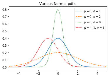
Definitely my most favorite distribution of all is the normal distribution.
\[f(x | \mu, \sigma) = \frac {1}{\sqrt{2\pi} \sigma} exp \left( - \frac {(x - \mu)^2}{2\sigma^2} \right)\]Here is the code:
Here is how it looks like:
Difference between:
- Normalization
- Standardization
The Central Limit Theorem
The central limit theorem simply put states that:
The average of the sample means will always be the population mean.
For further exploration:
- scipy.stats
- Introduction to Probability
Hypothesis and Inference
Hypothesis Testing
Confidence Interval
Bayesian Inference
A better alternative to hypothesis testing is the doing a Bayesian Inference procedure. This is done by interpreting probabilities not from the test but from the parameters themselves. This a bit technical on distributions we call beta (\(\beta\)) Distributions
(to be continued)
Needs more context and info
Want to collaborate? Message me in LinkedIn.
Here are my resources:
References
[1] Joel Grus. Data Science from Scratch: First Principles with Python.
[2] something. something. Retrieved from: something
[3] something. Retrieved from: something
[4] something. something. Retrieved from: something
[5] something. something. Retrieved from: something
[6] something. something. Retrieved from: https://epjdatascience.springeropen.com/articles/10.1140/epjds/s13688-019-0183-y
[7] something. something. Retrieved from : something